Reinforcement Learning with a Pick and Place Robotic Arm
tldr
I created a custom robotic arm environment where the arm is rewarded if it sorts shapes a certain way, and then punished if it knocks them off a table. I used OpenAI’s PPO method to be somewhat successful. If you want to skip to the code, go here.

The why
Reinforcement learning is a topic that’s endlessly fascinating to me. I had great success working through Deep Reinforcement Learning in Action, creating a generic Deep Q solver for several classic OpenAI gym environments. (You can find my work on that here). Observe terrified astronauts as HAL takes control and attempts to get them to the surface of the moon:
This was fun, but I wanted to try and get a closer to real-life applications of the tech. When my robotics reinforcement learning class came to a close, I really wanted to do the final project with a realistic robotics-oriented task. I also wanted to try a continuous action space problem, since my established knowledge of reinforcement learning was completely around discrete action spaces. With less than 3 weeks to do a complete project, I got to work.
Worlds to choose
I began looking for virtual environments I could get a quasi-realistic setup. I found numerous environments recommended for OpenAI’s gym, a python library created to create a generic interface for experimenting with RL techniques. Unfortunately OpenAI abandoned gym ages ago (OpenAI generally abandoned most of their robotics and RL research in favor of their language models, for better or worse). A new group created gymnasium, an open source port that is still maintained, while trying to maintain the same interface. It’s a great project, but this is just the symptom of a problem with a lot of RL work - specifically, a lot of environments aren’t well maintained.
Many of the environments that I came across was a pain to get working, requiring deprecated Python versions like 3.6 or deprecated versions of gym (and not compatible with gymnasium). Even while utilizing custom virtual environments for Python, installing the older versions (which can be a pain to get running by themselves) there tended to be bugs a lot of buggy environments. What seems to be the case with academic-focused code is that once the project is debuted and the paper submitted, there is little incentive to continue to support the endeavor. Of course I say this with my own open source work getting similar treatment. Pot, kettle, black, etc.
Below I list a few of the cooler environments I found that maybe you can use for your own RL projects, but keep in mind that some of them are going to require some elbow grease to get running. Similarly, if you aim to do this kind of work yourself, expect there to be headaches early in getting the environments to run. Considered environments were:
- Dexterous Hands - an extremely cool simulator based off of OpenAI’s dexterity robotics research.
- Dexterous Gym - similar to the above, with an additional paper for reference.
- IKEA Furniture Building - utilize various robotic arm platforms to try and assemble IKEA furniture, created for evaluating learning algorithms.
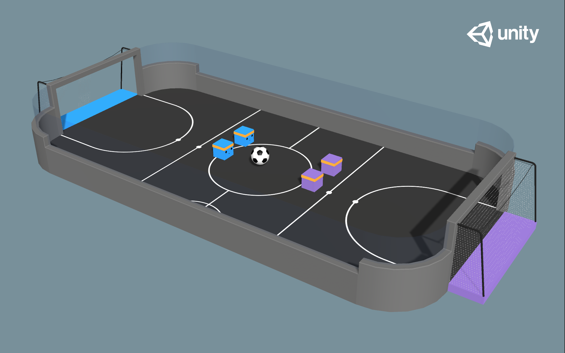
- Unity Learning Environments - More game-oriented, which would be fine if it wasn’t for my preference of a robotics-oriented focus. Also it’s been awhile since I’ve done anything in C++ or Unity, so it would require significant effort to ramp back to a productive level with it.
- Panda-Gym - a
gymstyle library based off of the collaborative 7-axis Panda robot arm, it presents several pre-made tasks and had good support for custom building your own environment. It was built onpybulletwhich meant I could tap into some physics engine features too like collision detection.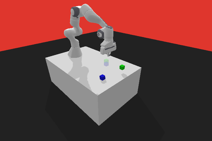
…and many, many more.
A fully custom environment was an option as well. As long as the environment can simulate a realistic robotic scenario and be controllable/configurable for repeated automated usage it’s an option. I looked into possible using Webots, Gazebo via ROS, and PyBullet to create a custom environment. Our three week timeline and my complete lack of skill in modeling meant that I couldn’t realistically pursue this avenue. I had created multiple custom environments in Pygame but I’m not sure you can do 3d in Pygame, and I’d have to code the entirety of a physics engine. Eep.
One driver for eliminating some environments was also a strong desire to try to do an RL project entirely consuming just camera inputs instead of state environment variables (essentially directly inputting key state values to the agent). I’ll talk more about where this went awry real quick later, but for now know that it was a factor in my choice.
In the end I selected Panda-Gym as it allowed me to create a more complicated/interesting environment without much headache, was relatively easy to get running, and I figured out a way to easily rip a “camera” view for image output. With the timeline in mind it seemed to strike an excellent balance.
Building our environment(s)
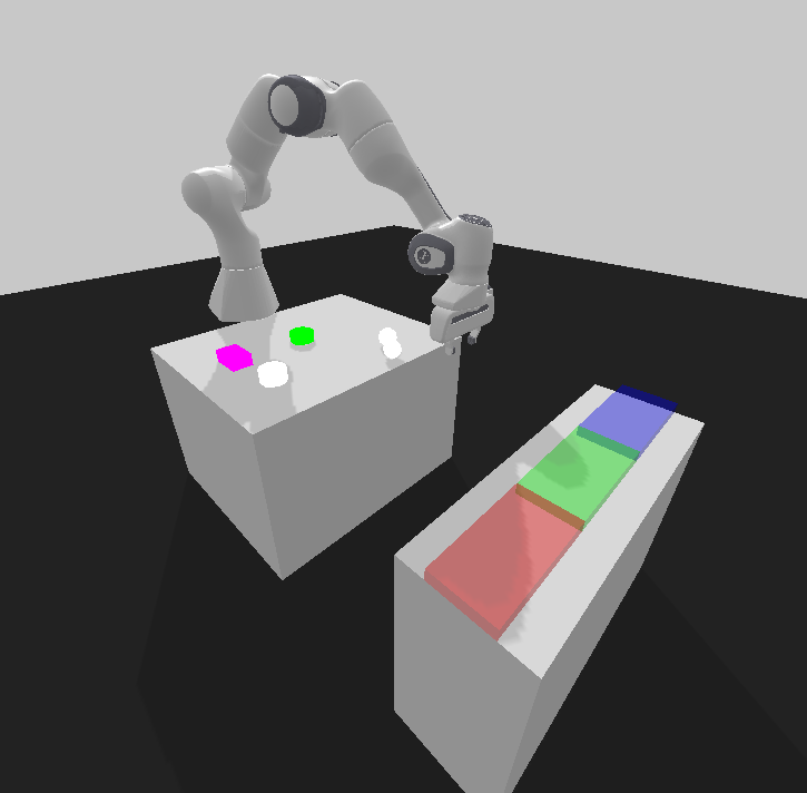
The panda-gym module was written from the start assuming you’d want to create your own custom environment, which was useful from the get-go. For the application I decided to try something simple - a pick and place environment. To avoid having to model anything I chose the objects to be randomly generated shapes (cubes, cylinders, and and spheres), and for the placement I wanted to have a set of “bins” that would reward you for placing the right shape into the right place.
So I went and began to construct through code my environment. A few hours later I have something resembling a pretty good setup, complete with randomized color, sized, and type of shapes to move. The “bins” are just transparent colored “zones” that detect collision with a block; when they do so, they remove the block and reward a set amount of points based on whether or not the block collided with the “correct bin”. I’ll expand more on reward design later.
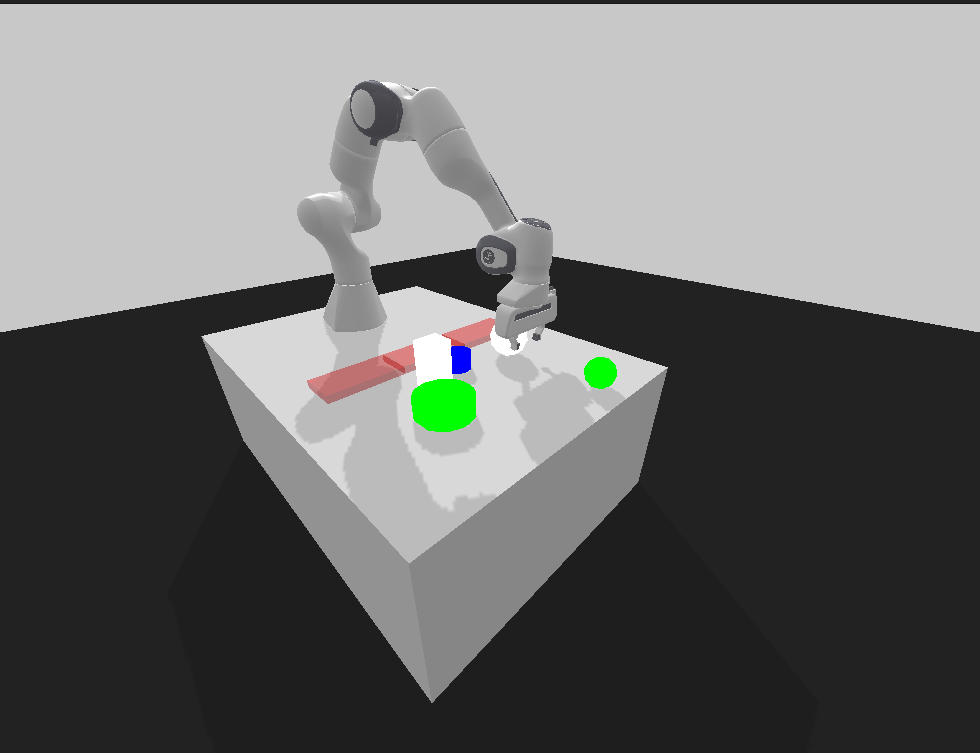
This was easy enough that I felt inspired. I actually created a second environment - what if we were successful and could do more complicated environments? Kind of like a stretch goal for the project? (Oh what poor misguided optimism). To that end I remembered a cool Google tossing robot task; why not try for that too? Thus I created a new environment with a deeply increased sense of difficulty labeled the “tosser” environment.
I mentioned before of the reason I chose panda-gym was my ability to grab the “view” as a sort of psuedo-camera. I created a class that would initialize both simulated robot and environment, and allow extraction of the camera view as an image array that I could feed into a network directly.
After building out the environment and image output I made sure to plug into panda-gym and its underlying pybullet engine to detect certain events. If the target objects are knocked off the table and hit the floor, I want to heavily penalize the agent. If they make contact with a “bin”, I want to reward the agent, but more-so if it was “correctly” sorted. Finally, I would include a penalty for each timestep, so that the agent would be penalized/rewarded for its relative urgency to action. While I would experiment later with changing these scores (trying to use reward shaping to finagle the behavior I wanted out of it), I ultimately settled on approximately the following:
| Event | Reward |
|---|---|
| Timestep | -1 |
| Object hits floor | -10 |
| Object reaches a bin | 25 |
| Object reaches the correct bin | 100 |
I then made the environment so it could be set to spawn a set number of objects on the table (though the objects would be sized, colored, and shaped randomly). Finally I added a configurable “blocker bar” - a black bar that would block the bins slightly, making simply sliding the blocks into the bins a bit harder to try and encourage lifting (spoiler: this theory didn’t work out).
One more thing to note - panda-gym actually has two modes of control - either controlling the movement of the end-effector by directly applying a delta in the X, Y, or Z planes, and giving a torque to apply to the end effector’s fingers. Inverse kinematics would be applied to determine what movement on the motors would be required to perform the action. Alternatively, it offered to take 8 torques as control input - a torque applied to each of its 7 joints and its fingers. This would allow for a greater range of motion, but the end-effector focused control would be simpler and likely easier to train. I created support for both, but ultimately trained just for the end-effector control.
Next I had to figure out how to control the arm since there was a serious twist to my prior efforts - the arm was a continuous action space.
Action movies spaces
An action space is the realm of possible actions that the agent can perform at a given timestep. A discrete action space, which encompasses all of the Deep Q projects I worked on in the past, has a predefined set of possible choices presented to the agent. Imagine an agent in an orthogonal maze, where you have a limited set of possible movement directions in every timestep… or a game where the agent can only generate button inputs for a joystick controller.
A continuous action space is a realm of possible values that fall within a potentially infinite range. Imagine the motor torques applicable to the wheels or joints of a robot. Even if there is a limited range of torque applicable - from zero to the max torque of the motor - there are still infinite possible decimal values within the given range. Even considering that there is a minimum resolution of enactable change (ie the motor controller can really only provide differences in the range of some minimum change, like, say, ±0.1 volts) there are so many possible values in that range of outputs that its effectively infinite.
So how do we approach a continuous action space? My initial hunch was maybe splitting the range of motions up into a set of possible intervals to create a pseudo-discrete action space. This fails in situations where the range of available space is variable, but the torque ranges possible on a robotic arm joint is typically constant. This quickly becomes messy though, with thousands of interval choices per motor - less than ideal. How can we maintain a continuous output?
With some research, we found a few approaches. The two most common seem to fall into two camps. We could either have a network directly output values for each expected output (and scale appropriately to the range if not infinite), or create a probability distribution for each output and have the network output the parameters of the distribution. The former is more straightforward, but the latter has the benefit of built-in exploration. Deep learning frameworks have various fully differentiable distribution layers that you can feed prior layer outputs in as parameters and can easily handle backpropagation through them.
Next - deciding how exactly we would train the arm.
Learning how to learn
I couldn’t utilize what I had used earlier in my deep Q learning projects. In these projects the network I trained is solving for the Q-value function Q(S,a) which is the resulting expected score of the given state and the determined action. An exploitative policy of picking the highest scoring state/action combinations over time in a well trained network should lead to a successful outcome.
In this approach we’re not training the policy directly - we’re solving for the value of a set of actions. Since we have an infinite number of actions, we’re not able to simply calculate all possible Q-values. We’re instead training the output policy directly, so tricks we learned before with Deep-Q learning such as experience replay or target networks are no longer applicable.
So with this goal in mind, I began researching different approaches.
First I looked into Deep Deterministic Policy Gradients (DDPG) (2015) from Google Deepmind. This work utilized an actor-critic approach - the actor is our policy network controlling our agent, and the critic estimates a value function utilized to calculate the value function to determine how good an action is. The actor network utilized in the initial paper is deterministic (directly outputting the action values). In time it was clear that DDPG was subject to overestimation biases (over inflating the value of certain state-action pairs) and was highly sensitive to hyperparameter tuning, making it difficult to train and apply to real world situations.
Deep Mind later came out with Twin Delayed Deep Deterministic Policy Gradients (TD3) (2018) to address these issues. It introduced an additional Q-value network critic (hence “twin”), using the smaller of the estimated values from the networks for its Bellman error loss functions. The policy actor network is updated less often than the value function critic network (approximately 2:1 but how often is a hyperparameter). Finally TD3 adds additional noise to target actions for exploration and to reduce exploitation of biased Q-value functions. These changes substantially improved performance over DDPG.
Meanwhile we also have Vanilla Policy Gradient, which is better known as REINFORCE. This was an older contribution before the deep learning/neural network revolution and is more of a generic approach with any function approximation method. Here we see the utilization of distribution functions/layers to output the policy.
OpenAI improved on REINFORCE with Trust Region Policy Optimization (2015), specifically citing robotic applications and demonstrating their algorithm on them - swimming, walking gaits - as well as some Atari games. (Note: TRPO can be used with discrete action spaces too, but we’re not focusing on that).
Not much later OpenAI released Proximal Policy Optimization (PPO) (2017). PPO promised improved performance over TRPO while simplifying its approach. It’s more sample efficient than TRPO, proved to be less sensitive to hyperparameter tuning, and has a feature known as a clipped objective which makes it easier to implement (tldr; eliminates the need to calcultae some extra derivatives). The clipped objective also ensures that we don’t see large updates to the policy network at once. The result - PPO is touted as an easy to implement and more effective alternative to TRPO.
So how do I choose? This took reading a number of forums, sample implementations, project blogs… anything that I could get my hands on. The rule of thumb seemed to come down to sample efficiency - how many instances of exploration in the environment does it take for the algorithm to learn complex tasks? While PPO was more sample efficient than TRPO, it still takes significant more than DDPG. Thus - if your environment is expensive to sample from (IE - you’re using real hardware and can’t simulate, or simulation is computationally expensive/unrealistic) use DDPG, otherwise use PPO as it’s easier to build and more robust to hyperparameter tuning.
With a deadline looming just three weeks away, it’s hard to argue with easier.
Why build?
Before going further, I want to address why I would build out this trainer from scratch when there are already libraries that will handle this for you while implementing state of the art techniques (such as Stable Baselines).
I wanted to build it from the ground up to prove that I understood each piece without a library hiding implementation details. Sure I’m using PyTorch, but I’ve built backpropagation from scratch and that’s not the core focus here. Likewise I wanted to be sure that I could apply these skills to a real robotic application and can realistically and confidently say “sure, I can build that” at some point in the future.
Blinding ourselves
I started building models that could take in one or multiple images. The idea with multiple images was less multiple camera views (something I didn’t yet bake into the environment but was area it might become necessary), but rather to try to give the model a concept of velocity for the blocks. I built this out, but then started to review the research I found.
While yes, some of the examples did use direct image input (such as the Atari games), most of the robotic environments were fed state variable input (relevant information pumped directly into the model). Those that did utilize images as direct input mentioned large distributed training, which I didn’t really have access to (we’ll discuss that later, actually).
It was clear that if I was going to pursue image input to the networks then it would take a significant amount of work and training time as well as significant compute resources. Given the tight deadline and my lone NVIDIA 3080 for training, it was clear that I was going to have to sacrifice that goal and swap over to a state variable input to simplify.
I made modifications to the environment to swap the output from image to state variables. What does our new input look like?
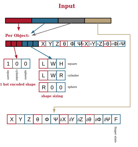
The environment would be preconfigured to have a set number of shapes (N) created at the start. Based on this value, the environment would have N sections of an 18 length vector. The first three values of the vector would be a one-hot encoded assignment of the shape type (square, cylinder, circle). The second set of three values would be the dimensions of the shape, depending on its shape type. Finally a set of 12 values representing the position, rotation, and then positional and rotational velocities of the shape were input. This information can be acquired perfectly in the simulation, and in the real world the information could be gleamed from overhead cameras tracking the objects. After each object vector, there would be a final vector representing the end effector’s position, rotation, positional and rotational velocities, and finally the finger torque.
Since I would change the number of objects throughout the project, the input size for the network would constantly change. All of the code had to be able to adapt to this variable input size throughout.
Starting out
We’re going to start looking at how I implemented code, so feel free to spy on the final results on the project’s GitHub repository.
I immediately started to work on the model and trainer. The model was easy. First I chose PyTorch over Tensorflow - I alternate between the two constantly in my own projects as both are good to know. Professionally I’ve only worked with Tensorflow, but I tend to lean towards PyTorch when I know I’m going to need to have a heavily customized training loop. (I also very much appreciate the object-oriented nature that PyTorch lends itself to).
I created a base class to encapsulate the agent called Actor and one called Critic. Both followed the same pattern, extending the PyTorch Module class and implementing instantiation, forward pass functionality, and for ease of use save and load functions.
The input size of the model is determined by what our observation size is like. Here I’m using the environment’s observation shape, but in some instances in the repository you may notice some hard coded sections as I experimented with different approaches. Ultimately, The first layer of the net is just the size of your observation, which we discussed earlier. The output layer similarly is the expected output shape of the environment as well.
class Actor(Module):
    def __init__(
        self,
        env: Any,
    ):
        self.input_size = env.observation_space["observation"].shape[0]
        self.output_size = env.action_space.shape[0]

        super(Actor, self).__init__()

        self.__initialize_model__()

    def __initialize_model__(self):
        # Create our model head - input -> some output layer before splitting to
        # different outputs for mu and sigma
        self.model = Sequential(
            Linear(self.input_size, 1024),
            LeakyReLU(),
            Linear(1024, 512),
            LeakyReLU(),
            Linear(512, 256),
            LeakyReLU(),
            Linear(256, 128),
            LeakyReLU(),
            Linear(128, 64),
            LeakyReLU(),
            Linear(64, 32),
            LeakyReLU(),
            Linear(32, self.output_size),
        )

        self.cov_var = torch.full(size=(self.output_size,), fill_value=0.5)
        self.cov_mat = torch.diag(self.cov_var)

    def forward(self, input: Union[np.ndarray, Tensor, List]) -> MultivariateNormal:
        if isinstance(input, np.ndarray):
            input_tensor: Tensor = torch.from_numpy(input.astype("float32"))
        elif type(input) is list:
            input_tensor: Tensor = torch.from_numpy(np.array(input).astype("float32"))
        else:
            input_tensor = input

        output = self.model(input_tensor)

        distribution: MultivariateNormal = MultivariateNormal(output, self.cov_mat)

        return distribution

    def save(self, filepath: str):
        torch.save(
            {
                "model": self.model.state_dict(),
            },
            filepath,
        )

    def load(self, filepath: str):
        data = torch.load(filepath)
        self.model.load_state_dict(data["model"])
The MultivariateNormal is a normal distribution function that outputs random outputs for multiple variables. Per the PPO paper we feed it a covariance matrix (a square matrix that describes the relationships between the variables). we set it at a diagonal of 0.5 which dictates that our output variables are uncorrelated. Sine it’s static, we don’t need to worry about it as it won’t change during training.
The critic model followed the same pattern, but had a different internal structure for the neural net.
self.model = Sequential(
    Linear(self.input_size, 128),
    LeakyReLU(),
    Linear(128, 64),
    LeakyReLU(),
    Linear(64, 32),
    LeakyReLU(),
    Linear(32, 1),
)
Note that we left the last layer of the critic unbounded, without a specified activation function, allowing us essentially a range of ±∞.
All other layers we keep as ReLU layers as a safe default choice. Our neural networks thus look like:
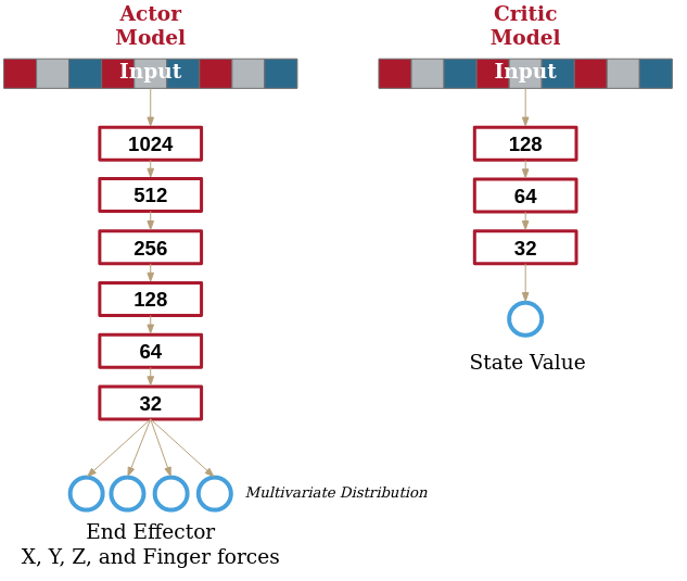
Building the trainer
Next up is building our trainer. The final version we’ll be looking at is in pose_trainer.py. I created a simple class to encompass the trainer to handle state management, and built in standard features - plot generation for progress, save and load functions, and a print_status function to output training progress from the terminal. Save functions would serialize configuration options, training state, and would in turn call save functions of passed models as well.
Where possible, I tried to break the training process into small bite-sized chunks so it’s easy to see what’s expected at each stage. In too many sample implementations I found training code was one gigantic block poorly explained and tough to track, so I aimed to do it as clearly as possible. I’m going to present overall what the trainer is doing, going into individual steps, and will finally show the finished training functions.
Knobs and levers
Configuration options ranged from PPO hyperparameters to trainer-specific settings. Expected hyperparameters you’d see in PPO implementations are:
| Hyperparameter | Typical Values | What is it? |
|---|---|---|
| γ | 0.95-0.99 | γ is commonly used in RL - it represents the discount factor weighing the importance of immediate rewards versus future rewards |
| ε | 0.2 | ε is not the same as in other RL applications; it’s not part of an epsilon-greedy approach, but rather defines the range within which updates are clipped - more on this later |
| α | 0.0003 | Learning rate |
| training_cycles_per_batch | 5 | How many times do we train on each generated batch? |
The process
Let’s review the expected steps of training an agent with PPO. Until we have trained a desired number of training steps (or reached a set of desired performance):
-
Perform a rollout - basically run the current model through as many episodes as needed until we reach a desired number (our desired batch size) in timesteps. We’ll expand on the rollout later.
-
Perform a training step
training_cycles_per_batchtimes. In each training step we’ll calculate the loss and perform backpropagation. -
Save the progress if you want; we did it at a configurable interval of timesteps.
That’s it! The devil is certainly in the details, but at a high level PPO can be quite simple.
Rollout
Let’s dig into the rollout. During the rollout, we expect to:
- Initialize memory to hold all of our:
observations- what was our state prior to taking an action?actions- what was the action of our arm in response to that observation?rewards- what was the reward at this step?log_probabilities- since we’re using probability distributions in our policy actor agent to generate our actions, we query the distribution for the log probability of the chosen action occurring. We need this for our loss function (discussed later)
- As long as we don’t have the desired total number of timesteps, run an entire episode - reset the environment, generate random shapes on the table, and see if our arm can collect them. Once the episode is finished (either by timeout or all shapes being removed) record each value we spoke of before and append them to our memory.
Here’s our rollout code where we perform each of these steps:
def rollout(self) -> EpisodeMemory:
    """
    rollout will perform a rollout of the environment and
    return the memory of the episode with the current
    actor model
    """
    observations: List[np.ndarray] = []
    log_probabilities: List[float] = []
    actions: List[float] = []
    rewards: List[float] = []

    while len(observations) < self.timesteps_per_batch:
        self.current_action = "Rollout"
        obs, chosen_actions, log_probs, rwds = self.run_episode()
        # Combine these arrays into our overall batch
        observations += obs
        actions += chosen_actions
        log_probabilities += log_probs
        rewards += rwds

        # Increment our count of timesteps
        self.current_timestep += len(obs)

        self.print_status()

    # We need to trim the batch memory to the batch size
    observations = observations[: self.timesteps_per_batch]
    actions = actions[: self.timesteps_per_batch]
    log_probabilities = log_probabilities[: self.timesteps_per_batch]
    rewards = rewards[: self.timesteps_per_batch]

    return observations, actions, log_probabilities, rewards
Here we see our run_episode function - note that check to seel the reset return to be compatible between our environment and the pendulum environment when we were debugging:
def run_episode(self) -> EpisodeMemory:
    """
    run_episode runs a singular episode and returns the results
    """
    observation, _ = self.env.reset()
    if isinstance(observation, dict):
        observation = observation["observation"]

    timesteps = 0
    observations: List[np.ndarray] = []
    actions: List[np.ndarray] = []
    log_probabilities: List[float] = []
    rewards: List[float] = []

    while True:
        timesteps += 1

        observations.append(observation)
        action_distribution = self.actor(observation)
        action = action_distribution.sample()
        log_probability = action_distribution.log_prob(action).detach().numpy()
        action = action.detach().numpy()
        observation, reward, terminated, _, _ = self.env.step(action)
        if isinstance(observation, dict):
            observation = observation["observation"]

        actions.append(action)
        log_probabilities.append(log_probability)
        rewards.append(reward)

        if timesteps >= self.max_timesteps_per_episode:
            terminated = True

        if terminated:
            break

    # Calculate the discounted rewards for this episode
    discounted_rewards: List[float] = self.calculate_discounted_rewards(rewards)

    # Get the terminal reward and record it for status tracking
    self.total_rewards.append(sum(rewards))

    return observations, actions, log_probabilities, discounted_rewards
Discount double check
One thing to note - when we finish running the episodes, we calculate at the end the discounted rewards instead of using the raw rewards. Using our assigned γ value, we include the future reward discounted by γ for each step back. This very common move allows the agent to understand future rewards while simultaneously valuing quicker solutions over longer ones.
def calculate_discounted_rewards(self, rewards: List[float]) -> List[float]:
    """
    calculated_discounted_rewards will calculate the discounted rewards
    of each timestep of an episode given its initial rewards and episode
    length
    """
    discounted_rewards: List[float] = []
    discounted_reward: float = 0
    for reward in reversed(rewards):
        discounted_reward = reward + (self.γ * discounted_reward)
        # We insert here to append to the front as we're calculating
        # backwards from the end of our episodes
        discounted_rewards.insert(0, discounted_reward)

    return discounted_rewards
Step by step
We have generated our batch, and want to perform a training “step” on it - calculate the loss and perform backpropagation on the model. First we’ll need to calculate the normalized advantage. The advantage is a measure of how much better or worse a given action is at a given state compared to the average action. To find this we utilize the critic model we’re training. We feed the critic the observations we recorded during our rollout and find out the expected advantage for each observation. We the normalize it by subtracting the mean and dividing by the deviation. You’ll note an extra 1e-8 to the denominator to prevent any ugly divide by zero errors.
def calculate_normalized_advantage(
    self, observations: Tensor, rewards: Tensor
) -> Tensor:
    """
    calculate_normalized_advantage will calculate the normalized
    advantage of a given batch of episodes
    """
    V = self.critic(observations).detach().squeeze()

    # Now we need to calculate our advantage and normalize it
    advantage = Tensor(np.array(rewards, dtype="float32")) - V
    normalized_advantage = (advantage - advantage.mean()) / (advantage.std() + 1e-8)

    return normalized_advantage
Once we have the normalized advantage, we need to calculate a ratio as per the PPO paper. This ratio’s goal is to estimate how much the new policy deviates from the old policy. By checking this ratio and clipping it, we can limit the total change in our policy to prevent large swings during training. The ratio is calculated as:
$$ \frac{\pi_\theta(a_t | s_t)}{\pi_{\theta_k}(a_t | s_t)} $$
…but we can take advantage of a trick to make it easier to compute and work with backpropagation. Specifically:
$$ \frac{a}{b} = e^{log(a) - log(b)} $$
We then take the minimum of the ratio by our normalized advantage or value clamped by some value from our hyperparameter ε:
$$ min( ratio, clamp( 1 - \epsilon, 1 + \epsilon, ratio ) ) $$
…where clamp is a min/max function for our given ratio. So if our ε is 0.2, the change is our ratio within a range of 0.8 to 1.2. Our actor loss is the average of this clamped ratio by the normalized advantage across all experienced states by our agent.
Next we calculate our critic loss - we simply using the mean squared error loss from what our discounted rewards were versus what the critic model predicted.
It’s all brought together here:
def training_step(
    self,
    observations: Tensor,
    actions: Tensor,
    log_probabilities: Tensor,
    rewards: Tensor,
    normalized_advantage: Tensor,
) -> Tuple[float, float]:
    """
    training_step will perform a single epoch of training for the
    actor and critic model

    Returns the loss for each model at the end of the step
    """
    # Get our output for the current actor given our log
    # probabilities
    current_action_distributions = self.actor(observations)
    current_log_probabilities = current_action_distributions.log_prob(actions)

    # We are calculating the ratio as defined by:
    #
    #   π_θ(a_t | s_t)
    #   --------------
    #   π_θ_k(a_t | s_t)
    #
    # ...where our originaly utilized log probabilities
    # are π_θ_k and our current model is creating π_θ. We
    # use the log probabilities and subtract, then raise
    # e to the power of the results to simplify the math
    # for back propagation/gradient descent.
    # Note that we have a log probability matrix of shape
    # (batch size, number of actions), where we're expecting
    # (batch size, 1). We sum our logs as the log(A + B) =
    # log(A) + log(B).
    ratio = torch.exp(current_log_probabilities - log_probabilities)

    # Now we calculate the actor loss for this step
    actor_loss = -torch.min(
        ratio * normalized_advantage,
        torch.clamp(ratio, 1 - self.ε, 1 + self.ε) * normalized_advantage,
    ).mean()

    self.actor_optimizer.zero_grad()
    actor_loss.backward()
    self.actor_optimizer.step()

    # Now we do a training step for the critic

    # Calculate what the critic current evaluates our states as.
    # First we have the critic evaluate all observation states,
    # then compare it ot the collected rewards over that time.
    # We will convert our rewards into a known tensor
    V = self.critic(observations)
    reward_tensor = Tensor(rewards).unsqueeze(-1)
    critic_loss = MSELoss()(V, reward_tensor)

    self.critic_optimizer.zero_grad()
    critic_loss.backward()
    self.critic_optimizer.step()

    return actor_loss.item(), critic_loss.item()
All together…
Now that we’ve talked about each piece, we can finally look at the total training function and understand each step it takes. Note that there is one more addition - we perform the training step multiple times per self.training_cycles_per_batch before running another rollout.
def train(self):
    """
    train will train the actor and critic models with the
    given training state
    """
    while self.current_timestep <= self.timesteps:
        # Perform a rollout to get our next training
        # batch
        observations, actions, log_probabilities, rewards = self.rollout()

        # Finally, convert these to numpy arrays and then to tensors
        observations = Tensor(np.array(observations, dtype=np.float32))
        actions = Tensor(np.array(actions, dtype=np.float32))
        log_probabilities = Tensor(np.array(log_probabilities, dtype=np.float32))
        rewards = Tensor(np.array(rewards, dtype=np.float32))

        # Perform our training steps
        for c in range(self.training_cycles_per_batch):
            self.current_action = (
                f"Training Cycle {c+1}/{self.training_cycles_per_batch}"
            )
            self.print_status()

            # Calculate our losses
            normalized_advantage = self.calculate_normalized_advantage(
                observations, rewards
            )
            actor_loss, critic_loss = self.training_step(
                observations,
                actions,
                log_probabilities,
                rewards,
                normalized_advantage,
            )
            self.actor_losses.append(actor_loss)
            self.critic_losses.append(critic_loss)

        # Every X timesteps, save our current status
        if self.current_timestep - self.last_save >= self.save_every_x_timesteps:
            self.current_action = "Saving"
            self.print_status()
            self.save("training")

    print("")
    print("Training complete!")

    # Save our results
    self.save("training")
Training struggles
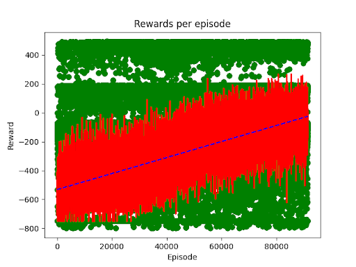
Unfortunately things were not smooth sailing at first. We started out with a busy table of 5 objects and our blocker bar enabled. We tracked in the trainer’s state performance over time for tracking. Below is an early example of that feature. Here we have a plot of a given episode number by the rewards in that episode. Green dots represent a singular episode’s score, and the red line represents the average score of the last 100 episodes (to smooth it out). (Later versions of this chart we added a dotted blue line representing a regression fit on the points to look at overall trends from the first episode)
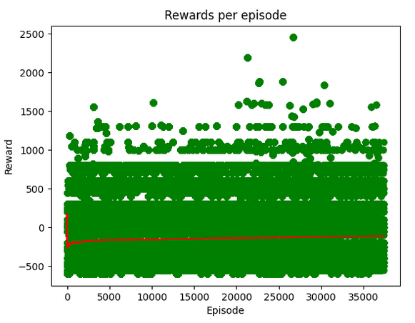
…as you can see, we had over 40k episodes with over 2 million timesteps (as a side note, while we measure episodes for easier data tracking, most papers tend to discuss learning over timesteps) we had no discernible learning going on. In the simulation the arm would just twitch or decide to do its best to avoid the task entirely.
This led to a lot of miniature experiments. First we needed to confirm that our model and trainer could learn anything. Since we followed the gym API format set out by OpenAI, we could mostly switch our setup towards a simpler environment. We chose the pendulum environment from the gymnasium module. It’s the simplest possible continuous action space environment, and only minor modifications to the model was needed to adapt it to the new dimensions of the input/output (beyond these layers I changed nothing else in the model).

A bit later we found that we still couldn’t learn, implying either the model was the issue (unlikely, given we found implementations of the pendulum environment with far fewer parameters) or we had an issue in our trainer. For example, here’s our pendulum after 2 million timesteps of training:
Ultimately we narrowed the issue down to the calculation of the loss function. The version I described above when discussing how it was built is actually the final version, with all fixes and adjustments included.
What was wrong in the trainer? First we noticed that our observations were being paired with our states… in the wrong order. Basically an off-by-one error. We then realized within the loss, where we calculate the log probabilities incorrectly which created wildly inaccurate losses. After adjusting these (and one or two late nights) learning was finally apparent! Our agent clearly learned after around 300k timesteps, with the scenario being “solved” after a few million timesteps.

When your reinforcement agent isn’t learning - simplify and try to predict and walk-through what expected losses should be. The benefit of following the gymnasium API that OpenAI’s gym popularized is we can always plug in these simpler environments. Similarly understanding each step of the loss process is crucial to ensure your backpropagation is going to work as you expect.
Diving back into our environment, we decided to simplify a bit as well - we shrunk down to one object and turned off the block bar just to see if we could get learning in our environment.

Here we saw definitive learning (improvement of average scores) after just 20k episodes, or about 1 million episodes. Slow, but still positive improvement. One thing that immediately became obvious that even though we saw learning, we also had a very high variance, evidenced by the arm occasionally just refusing to do more than just twitch about and our large spread of green dots in our chart.
So how can we speed up learning? Rereading the initial PPO paper and additional comments from various implementations we found two pieces of advice. The first was that a dense reward signal can have significant effect on learning. We were already applying rewards and penalties on most actions the arms were doing (so we didn’t have to worry about a sparse reward, like only rewarding a singular point at the end of the scenario or not). The best we could do was to amplify the signal a bit by adjust the scale of those awards. Thus our new reward scheme was:
| Event | Reward |
|---|---|
| Timestep | -1 |
| Object hits floor | -50 |
| Object reaches a bin | 200 |
| Object reaches the correct bin | 500 |
This showed some improvement on initial experiments, but not as significant as the next hyperparameter we tuned - batch sizes. We had originally approached the problem at about 10k timesteps per batch. We ran a gamut of testing from 5k timesteps per batch to 200k timesteps per batch. At the smaller 5k timesteps per batch we saw flat results with no learning, even worse than our original 10k. At 50k timesteps per batch we saw a noticeable improvement in learning. At 200k timesteps we saw an even larger jump in learning progress.
We utilized 200k timesteps per batch for the remainder of the project. Why not try higher? Scaling limits. I trained this project on a NVIDIA 3080 with 10 gigs of RAM and I was near maxing it - we couldn’t do larger batch sizes with my computer. Seeing as I didn’t want to spend a significant amount of money renting a larger machine (and as far as I could find there were no GPU clusters or services available to us WPI students). Not only that, but it took a significant amount of time to generate the necessary episodes to complete each batch (…since PPO generates a new batch on its freshly updated model) started to take too long - over ten minutes per batch.
By this point we’re down to less than a week and a half to go.
Not quite distributed training
This is a brief side-experiment I did on whether or not I could quickly modify the rollout to be distributed. Feel free to skip
What slowed us down significantly was the high cost of experimentation. Any experiment we put forward would require millions of timesteps to even begin to see significant learning, and that meant an overnight run of the simulator. The actual backpropagation of the batch sizes only took about 90 seconds, so optimizing the time to run rollout is the clear target. I wondered, with a few days to go, could I do a last minute distributed rollout feature?
The general idea - try to convert my rollout functionality into a standalone server that I could host in the cloud and see if there was affordable computation resources I could use to get a time reduction for each batch generation.
I started by throwing together a dockerfile to construct a custom docker image with Python and necessary libraries from the project. I created a little flask server that would accept a request to run a rollout complete with a copy of the model. I was under time pressure so I just quickly serialized the model to a binary payload. The docker image server would receive a call to with the model, deserialize it, load the model, and run a single episode of rollout. Once it was done it would return a large serialized binary payload of each timestep of the episode (we need all of them for backpropagation and loss calculations).
I loaded up Google’s GCP, specifically their Cloud Run service, which acts as a Function as a Service (FaaS) platform. Cloud Run will take our docker image and deploy it as a server at a set endpoint and handle authentication, scaling, and routing for us. I’ve used it before successfully in a number of applications in my own professional career. I created a deployment and tested it - and it worked on the first try!
I created a temporary replacement of our rollout function that created a configurable number of workers that would call out to the Cloud Run endpoint. I had configured the endpoint to run only one API call per server and had it set to scale to the number of workers I was having the trainer use - basically 1 worker per rollout.
This actually was shockingly easy. I had added timing metrics to the per-episode and per-batch rollout prior to my local version, and did the same on the new distributed rollout function. I set a dozen workers and fired off the test. The results? The rollouts were taking longer - much longer.
The possible causes of the delay? The new network call had to send the model and receive all of the episodes results - which actually made sizable payloads - with a not insignificant transport time. Serialization of the results was likely no small addition either. And possibly most importantly the processing power of Cloud Run instances by default are much lower than the desktop I was running on. I thought of this prior but thought if I ran enough workers it wouldn’t be an issue. Unfortunately from the time per episode I was seeing didn’t bode well - some quick back of the napkin math showed that I would need far too many instances to get the speedup I needed, or would need to pay for much more powerful instances.
…in either case the solution required a bit too much money I was willing to budget this project, especially since it wasn’t clear that the larger rollouts I wanted to do would actually reduce variance. With only 2 days to go by this point, I decided to be happy with what I had.
Results
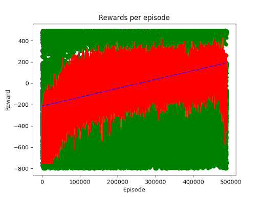
After three intense weeks of building, testing, debugging, and training, we had some okay results. We still had high variance in our trained models - occasionally the model routinely glitches and just refuses to work - but other times it quickly and efficiently slides the blocks to the appropriate bin. Here’s an example of the one object spawned at a time with our blocker bar enabled:

We can see a trend a performance trend upwards demonstrating learning despite the variance. It took almost 500k episodes, approximately 20 million timesteps.
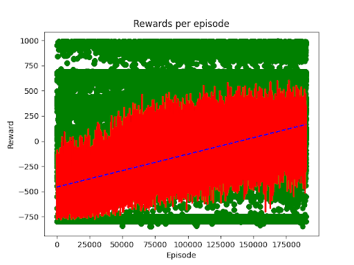
Another example we trained up used 2 objects and removed the blocker bar. You see in this example occasionally the arm freaks out, but can generally get 1 or 2 shapes quickly.

…though this was a shorter training session, just ~175k episodes for only about 35 million timesteps.
Acceptable and a great proof of understanding, even if it doesn’t perform quite how I envisioned.
Lessons learned
No project is complete without some reflection. What are the key points to remember when working with PPO? What would I do differently in future projects?
-
It takes millions of timesteps of training to just see learning begin; be ready for a long haul
-
Dense reward signal is crucial for complicated tasks - Utilize reward shaping as best as you can for the you want.
-
Batch size matters a lot - you should be looking at the many 10k’s of timesteps per batch if not 100k’s of timesteps
-
Build for distributed rollout from the beginning. Expect anything but toy examples to require hours of compute across multiple machines. Syncing models and getting observations back is costly over network, so spend time figuring out how to efficiently transport them.
Next Steps
I’d be lying if I said that I truly thought I was done with the original goal of this project - I still want to experiment with applying reinforcement learning to robotic applications. Despite the questionable performance attained in its final form, I think I might revisit the project some day and apply lessons learned. So what’s the next steps for if I do?
I probably will try to adapt the Stable Baseline PPO trainer to see if it experiences such high variance. If not, then I’ll have to dig through the different approaches in the trainers to try and determine what key differences are causing it.
Similarly a rebuilt trainer from scratch with a distributed trainer planned from the start would be interesting - can I get my batch size to millions of steps in this manner?
Finally, I’d modify the environments to have more direct reward shaping - specifically to reward holding/lifting the objects with the fingers to get more pick and place style movements.